Nickel Direct Imaging Data Reduction
Basis of this jupyter notebook is from Keerthi Vasan Gopala Chandrasekaran (UC-Davis), who created it from Elinor Gates' (UCO/Lick) 2018 Observational Astronomy Workshop python data reduction activity. Additional code contributions and conversion so it would work under Python 3 were from Azalee Bostroem (UC-Davis). Elinor Gates subsequently added commentary, expanded the code to make sure everything is done inside python, and added the cosmic ray rejection section. This is designed to work with Python 3.
If the data are properly acquired and FITS headers are accurate, this should work as a basic data reduction pipeline. However, proceeding slowly, one step at a time, examining calibration and image frames at each step is encouraged so that understanding of each step and its importance to the general data reduction is understood, as well as catching errors and implementing fixes as soon as possible in the procedures.
Import the Necessary Python Packages
from astropy.io import fits,ascii
import numpy as np
import sys, getopt,os
import glob2
Organize Data
All data should be in one directory initially. This can be any directory as the path to it will be set as the source_dir below. You'll want to change the source directory appropriately for your data location. Also, you should remove any bad frames (e.g. flat field frames with unacceptable properties, etc.) from the directory so they don't contaminate the reduced data. It is wise to keep a separate backup of the raw data incase there are problems and you need to start data reduction over from the beginning.
source_dir = '/Users/egates/Desktop/python3Test/'

# Location of the folder containing all the data files (bias, domeflats, twilight flats, and the data files)
f = source_dir + '*.fits'
Overscan Subtraction
The overscan region(s) are additional columns appended to the data that measure the overall bias values for each row at the time the data were acquired. Depending on the camera, these may be very stable over a night of observing, or vary from image to image. This bias level needs to be subtracted before further data reduction steps should be done. Overscan subtraction is done on all calibration and science files.
The original overscanLickObsP3.py code is available on-line via our optical instrument manuals will read a list of files in, determine the overscan and data regions for each file, fit the overscan, then subtract it from the data, writing out a new overscan subtracted image for each input image. This code is specific to Lick Observatory data and keywords, but could easily be altered with the appropriate keywords to work with other detectors with one or two amplifiers. The code below has been modified from the original to create input and output filelists according to the file directory denoted above. If you have a lot of data, this may take a few minutes to run.
def main(argv):

    # set fit = 'yes' to do legendre fit to overscan regions, 'no' to just use the median
    fit = 'yes'

    # create input and output file name lists.  Output files will have unique names, leaving the input files unchanged.
    ifilelist = glob2.glob(f)
    # _os stands for overscan subtracted in the output file names
    ofilelist = [i[:-5]+ '_os.fits' for i in ifilelist]

    # how many files
    numifiles = len(ifilelist)
    numofiles = len(ofilelist)
    if numifiles != numofiles:
        sys.exit('Input and output file lists have different numbers of files. Exiting.')

    # For each file in ifilelist, read in file, figure out overscan and data regions, fit
    # overscan with desired function (if any), and subtract from data.
    # Write data to ofilelist value.

    for i in range(0,numifiles):
        ifile=ifilelist[i]
        ofile=ofilelist[i]
        data, header = fits.getdata(ifile,header=True)

        # change data to float
        data=data.astype('float32')

        # read necessary keywords from fits header

        #number of pixels in image
        xsize = header['NAXIS1']
        ysize = header['NAXIS2']
        #start column and row
        xorig = header['CRVAL1U']
        yorig = header['CRVAL2U']
        #binning and direction of reading pixels
        cdelt1 = header['CDELT1U']
        cdelt2 = header['CDELT2U']
        #number of overscan columns
        rover = header['ROVER']
        cover = header['COVER']
        #unbinned detector size
        detxsize = header['DNAXIS1']
        detysize = header['DNAXIS2']
        #number of amplifiers
        ampsx = header['AMPSCOL']
        ampsy = header['AMPSROW']

        # determine number and sizes of overscan and data regions
        namps = ampsx*ampsy
        if rover > 0:
            over=rover
            sys.exit('Program does not yet deal with row overscans. Exiting.')
        else:
            over = cover
        if over == 0:
            sys.exit('No overscan region specified in FITS header. Exiting.')

        # single amplifier mode (assumes overscan is the righmost columns)
        if namps == 1:
            biassec = data[:,xsize-cover:xsize]
            datasec = data[0:,0:xsize-cover]

            # median overscan section
            bias=np.median(biassec, axis=1)

            # legendre fit
            if fit == 'yes':
                # fit
                lfit = np.polynomial.legendre.legfit(range(0,len(bias)),bias,3)
                bias = np.polynomial.legendre.legval(range(0,len(bias)),lfit)

            # subtract overscan
            datanew = datasec
            for i in range(datasec.shape[1]):
                datanew[:,i] = datasec[:,i]-bias

        # two amplifier mode (assumes both amplifer overscans are at rightmost columns)
        if namps == 2:
            biasseca = data[:,xsize-cover*2:xsize-cover]
            biassecb = data[:,xsize-cover:xsize]

            # median overscan sections
            biasa=np.median(biasseca,axis=1)
            biasb=np.median(biassecb,axis=1)

            # legendre fit
            if fit == 'yes':
                lfita = np.polynomial.legendre.legfit(range(0,len(biasa)),biasa,3)
                lfitb = np.polynomial.legendre.legfit(range(0,len(biasb)),biasb,3)
                biasa = np.polynomial.legendre.legval(range(0,len(biasa)),lfita)
                biasb = np.polynomial.legendre.legval(range(0,len(biasb)),lfitb)

            # Extract data regions

            # determine boundary between amplifiers
            bd=detxsize/2/abs(cdelt1)

            # calculate x origin of readout in binned units if cdelt1 negative or positive
            if cdelt1 < 0:
                #if no binning x0=xorig-xsize-2*cover, with binning:
                x0=xorig/abs(cdelt1)- (xsize-2*cover)
            else:
                x0=xorig/cdelt1

            xtest=x0+xsize-cover*2 # need to test if all data on one or two amplifiers

            # determine which columns are on which amplifier and subtract proper overscan region

            if xtest < bd: # all data on left amplifier
                datanew=data[:,0:xsize-cover*2]
                m=datanew.shape[1]
                for i in range(0,m):
                    datanew[:,i]=datanew[:,i]-biasa

            if x0 >= bd: # all data on right amplifier
                datanew=data[:,0:xsize-cover*2]
                m=datanew.shape[1]
                for i in range(0,m):
                    datanew[:,i]=datanew[:,i]-biasb

            if xtest >= bd and x0 < bd:  #data on both amplifiers
                x1=int(bd-x0)
                dataa=data[:,0:x1]
                datab=data[:,x1:-cover*2]
                ma=dataa.shape[1]
                mb=datab.shape[1]
                for i in range(0,ma):
                    dataa[:,i]=dataa[:,i]-biasa
                for i in range(0,mb):
                    datab[:,i]=datab[:,i]-biasb
                # merge dataa and datab into single image
                datanew=np.hstack([dataa,datab])

        if namps > 2:
            sys.exit('Program does not yet deal with more than two overscan regions. Exiting.')

        # add info to header
        header['HISTORY'] = 'Overscan subtracted'

        # write new fits file
        fits.writeto(ofile,datanew,header,overwrite=True)

if __name__ == "__main__":
   main(sys.argv[1:])
Organize Overscan Subtracted Files
Move all the overscan subtracted (e.g. the newly created *_os.fits) bias, data, and flat field files in separate folders, for example:

Below we set up paths for file sorting, and sort the files into the appropriate folders.
# Make the directories for this data reduction procedure
# I like to make an archive directory to store files that are no longer needed for the data reduction,
# but still available to examine if needed if there are issues with the data reduction.

biasdir = source_dir+'bias/'
datadir = source_dir+'Data_files/'
domeflatdir = source_dir+'flat_dome/'
twiflatdir = source_dir+'flat_twilight/'
archivedir = source_dir+'archive/'

os.mkdir(biasdir)
os.mkdir(datadir)
os.mkdir(domeflatdir)
os.mkdir(twiflatdir)
os.mkdir(archivedir)
# Make a list of all the overscan subtracted files
os_files = glob2.glob(source_dir+'*os.fits')

# Move calibration frames to appropriate directories
# In this case we are assuming that twilight flats have 'twi' in the OBJECT FITS header keyword,
# dome flats have 'dome' in OBJECT, etc.  If the names are different, you'll need to adjust the search strings
# for sorting the files.
for ifile in os_files:
    hdr = fits.getheader(ifile)
    basename=os.path.basename(ifile)
    if 'twi' in hdr['OBJECT'].lower():
        os.rename(ifile,twiflatdir+basename)
    elif 'dome' in hdr['OBJECT'].lower():
        os.rename(ifile,domeflatdir+basename)
    elif 'bias' in hdr['OBJECT'].lower():
        os.rename(ifile,biasdir+basename)
    else:
        os.rename(ifile,datadir+basename)
# Location of the folders and files for use later
f1 = source_dir + 'bias/*.fits'
f2 = source_dir + 'Data_files/*.fits'
f3 = source_dir + 'flat_dome/*.fits'
f4 = source_dir + 'flat_twilight/*.fits'
Create Master Bias File
The Master Bias file is the median combined bias frames. If the detector is particularly flat with no bias structure, this step may not be needed. In the case of the Nickel Direct Imaging CCD, there is significant bias structure that needs to be removed, so this step is necessary to remove that structure.
# Create list of bias files
biasfiles = glob2.glob(f1)
data_stack = []
for file in biasfiles:
    data_stack.append(fits.getdata(file))

# Median combine the bias files to create the Master Bias frame
medianBias = np.median(data_stack,axis=0)

# Write out the master bias file with updated FITS header information
header = fits.getheader(biasfiles[0])
header['HISTORY'] = 'Median combined'
fits.writeto(source_dir+'bias.fits',medianBias,header)

# Move the no longer needed overscan subtracted frames to the archive directory
for file in biasfiles:
    basename=os.path.basename(file)
    os.rename(file,archivedir+basename)
Check Master Bias File
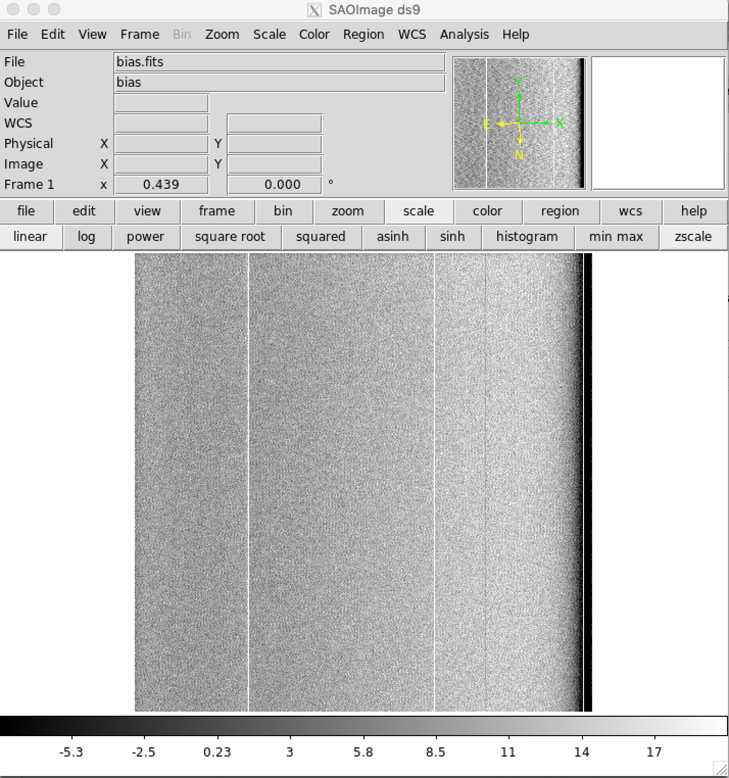
It is best to check the bias.fits file to make sure it looks OK before continuing. DS9 is a frequently used tool in astronomy for examining FITS images. DS9 is not a python tool, but freely downloadable for virtually all computer operating systems. Typical Nickel bias images look like the following.

Bias Subtract Flat Field and Data Frames
Because the files were sorted into subdirectories, we'll be doing essentially the same steps for the files in the Data_files, flat_dome, and flat_twilight directories.
# Bias subtracting the data files

# Make list of input bias files
datafilesin = glob2.glob(f2)

# _bs stands for bias subtracted in the output file names
datafilesout = [i[:-5]+ '_bs.fits' for i in datafilesin]

n = len(datafilesin)
for i in range(0,n):
    data,header = fits.getdata(datafilesin[i],header=True)
    dataout = data - medianBias
    header['HISTORY'] = 'Bias subtracted'
    fits.writeto(datafilesout[i],dataout,header)
    # Move the no longer needed overscan subtracted files to the archive directory
    basename=os.path.basename(datafilesin[i])
    os.rename(datafilesin[i],archivedir+basename)
# Bias subtracting the dome flat files

# Make list of input dome flat field files
datafilesin = glob2.glob(f3)

# _bs stands for bias subtracted in the output file names
datafilesout = [i[:-5]+ '_bs.fits' for i in datafilesin]

n = len(datafilesin)
for i in range(0,n):
    data,header = fits.getdata(datafilesin[i],header=True)
    dataout = data - medianBias
    header['HISTORY'] = 'Bias subtracted'
    fits.writeto(datafilesout[i],dataout,header)
    # Move the no longer needed overscan subtracted files to the archive directory
    basename=os.path.basename(datafilesin[i])
    os.rename(datafilesin[i],archivedir+basename)
# Bias subtracting the twilight flat files

# Make list of input twilight flat field files
datafilesin = glob2.glob(f4)

# _bs stands for bias subtracted in the output file names
datafilesout = [i[:-5]+ '_bs.fits' for i in datafilesin]

n = len(datafilesin)
for i in range(0,n):
    data,header = fits.getdata(datafilesin[i],header=True)
    dataout = data - medianBias
    header['HISTORY'] = 'Bias subtracted'
    fits.writeto(datafilesout[i],dataout,header)
    # Move the no longer needed overscan subtracted files to the archive directory
    basename=os.path.basename(datafilesin[i])
    os.rename(datafilesin[i],archivedir+basename)
Create Normalized Flat Field frames
For this example we will use the twilight flat field frames, as they are generally superior to dome flats. One uses dome flats if the twilight flat field frames were unattainable due to weather or there was some other technical issues. First we will create lists of files for each filter, then combine the frames to create the final normalized flat field frame for each filter.
# This assumes that the B, V, R, and I filters were used.  If different filters were used, you'll need to change the
# code below accordingly

# If you are using dome flat fields, rather than twilight flats, you'll need to change the code below to
# source the right directory of files and check the header OBJECT accordingly.

b_flist = []
v_flist = []
r_flist = []
i_flist = []

# Make list of all the flat field files in the twilight flat field directory
flatlist = glob2.glob(f4)

# Sort files into lists based on the filter used
for ifile in flatlist:
    hdr = fits.getheader(ifile)
    if 'twi' in hdr['OBJECT'].lower():
        filt = hdr['FILTNAM']
        if filt == 'B':
            b_flist.append(ifile)
        if filt == 'V':
            v_flist.append(ifile)
        if filt == 'R':
            r_flist.append(ifile)
        if filt == 'I':
            i_flist.append(ifile)
# Create the Master B Flat
bflat_stack = []

# Read in each file and normalize by the median
for file in b_flist:
    data,header = fits.getdata(file,header=True)
    data = data / np.median(data)
    bflat_stack.append(data)
    # Move the no longer needed files to archivedir
    # Move the now no longer needed files to archivedir
    basename=os.path.basename(file)
    os.rename(file,archivedir+basename)

# Median combine the flat fields, then normalize by the mean
bflat = np.median(bflat_stack,axis=0)
m = np.mean(bflat)
bflat = bflat/m
header['HISTORY'] = 'Combined and normalized flat field'
fits.writeto(source_dir + 'bflat.fits',bflat,header,overwrite=True)
# Create the Master V Flat
vflat_stack = []

# Read in each file and normalize by the median
for file in v_flist:
    data,header = fits.getdata(file,header=True)
    data = data / np.median(data)
    vflat_stack.append(data)
    # Move the no longer needed files to archivedir
    basename=os.path.basename(file)
    os.rename(file,archivedir+basename)

# Median combine the flat fields, then normalize by the mean
vflat = np.median(vflat_stack,axis=0)
m = np.mean(vflat)
vflat = vflat/m
header['HISTORY'] = 'Combined and normalized flat field'
fits.writeto(source_dir + 'vflat.fits',vflat,header)
# Create the Master R Flat
rflat_stack = []

# Read in each file and normalize by the median
for file in r_flist:
    data,header = fits.getdata(file,header=True)
    data = data / np.median(data)
    rflat_stack.append(data)
    # Move the no longer needed files to archivedir
    basename=os.path.basename(file)
    os.rename(file,archivedir+basename)

# Median combine the flat fields, then normalize by the mean
rflat = np.median(rflat_stack,axis=0)
m = np.mean(rflat)
rflat = rflat/m
header['HISTORY'] = 'Combined and normalized flat field'
fits.writeto(source_dir + 'rflat.fits',rflat,header)
# Create the Master I Flat
iflat_stack = []

# Read in each file and normalize by the median
for file in i_flist:
    data,header = fits.getdata(file,header=True)
    data = data / np.median(data)
    iflat_stack.append(data)
    # Move the no longer needed files to archivedir
    basename=os.path.basename(file)
    os.rename(file,archivedir+basename)

# Median combine the flat fields, then normalize by the mean
iflat = np.median(iflat_stack,axis=0)
m = np.mean(iflat)
iflat = iflat/m
header['HISTORY'] = 'Combined and normalized flat field'
fits.writeto(source_dir + 'iflat.fits',iflat,header)
Check Normalized Flat Field Frames
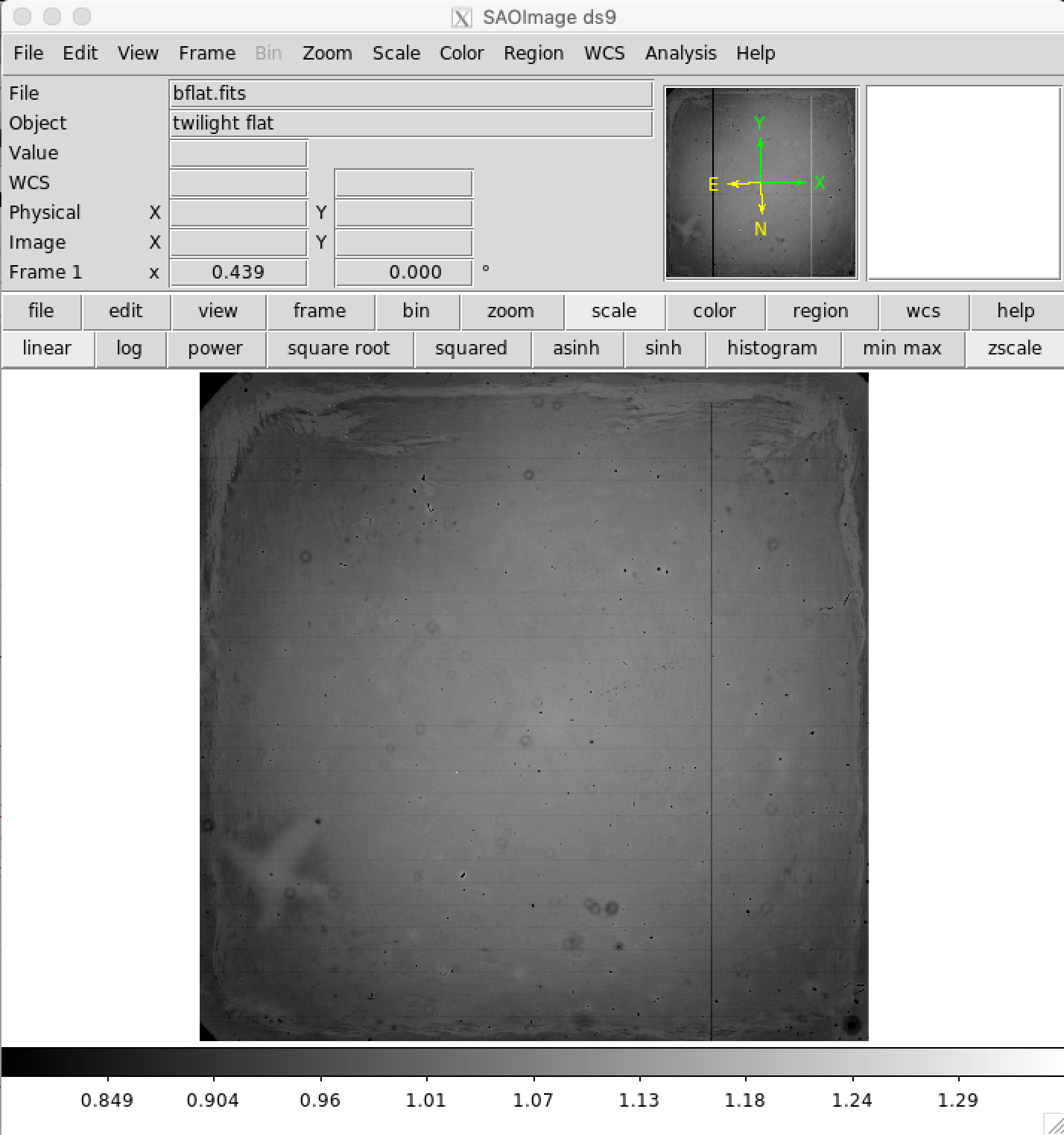
It is wise to check the normalized flat field frames using DS9 or similar tool. Most pixel values should be very close to 1.0. A typical B-band normalized flat field is shown as an example.

Flat Field Data Frames
Flat fielding data is an essential step in the data reduction to calibrate the relative sensitivies of each pixel. First the data files will be sorted based on their filters, then each frame divided by the appropriate filter normalized flat field file.
# Create lists of data files for each filter. Filter names should match the filter names used for creating the Flat
# Field lists of files.  Again, we are assuming B, V, R, and I filters were used.

b_flist = []
v_flist = []
r_flist = []
i_flist = []

# Make list of all bias subracted data files
data_flist = glob2.glob(f2)

# Sort data files by filter
for ifile in data_flist:
    hdr = fits.getheader(ifile)
    filt = hdr['FILTNAM']
    if filt == 'B':
        b_flist.append(ifile)
    if filt == 'V':
        v_flist.append(ifile)
    if filt == 'R':
        r_flist.append(ifile)
    if filt == 'I':
        i_flist.append(ifile)
# Flat Field the B data files

# _ff stand for flat fielded for the output file name
bdataout = [i[:-5]+ '_ff.fits' for i in b_flist]

# For each file in list, divide by the normalize flat field frame for that filter
n=len(b_flist)
for i in range(0,n):
    data,header = fits.getdata(b_flist[i],header=True)
    dataout = data / bflat
    header['HISTORY'] = 'Flat Fielded'
    fits.writeto(bdataout[i],dataout,header)
    # Move bias subtracted images to archivedir now that they are no longer needed
    basename=os.path.basename(b_flist[i])
    os.rename(b_flist[i],archivedir+basename)
# Flat Field the V data files

# _ff stand for flat fielded for the output file name
vdataout = [i[:-5]+ '_ff.fits' for i in v_flist]

# For each file in list, divide by the normalize flat field frame for that filter
n=len(v_flist)
for i in range(0,n):
    data,header = fits.getdata(v_flist[i],header=True)
    dataout = data / vflat
    header['HISTORY'] = 'Flat Fielded'
    fits.writeto(vdataout[i],dataout,header)
    # Move bias subtracted images to archivedir now that they are no longer needed
    basename=os.path.basename(v_flist[i])
    os.rename(v_flist[i],archivedir+basename)
# Flat Field the R data files

# _ff stand for flat fielded for the output file name
rdataout = [i[:-5]+ '_ff.fits' for i in r_flist]

# For each file in list, divide by the normalize flat field frame for that filter
n=len(r_flist)
for i in range(0,n):
    data,header = fits.getdata(r_flist[i],header=True)
    dataout = data / rflat
    header['HISTORY'] = 'Flat Fielded'
    fits.writeto(rdataout[i],dataout,header)
    # Move bias subtracted images to archivedir now that they are no longer needed
    basename=os.path.basename(r_flist[i])
    os.rename(r_flist[i],archivedir+basename)
# Flat Field the I data files

# _ff stand for flat fielded for the output file name
idataout = [i[:-5]+ '_ff.fits' for i in i_flist]

# For each file in list, divide by the normalize flat field frame for that filter
n=len(i_flist)
for i in range(0,n):
    data,header = fits.getdata(i_flist[i],header=True)
    dataout = data / iflat
    header['HISTORY'] = 'Flat Fielded'
    fits.writeto(idataout[i],dataout,header)
    # Move bias subtracted images to archivedir now that they are no longer needed
    basename=os.path.basename(i_flist[i])
    os.rename(i_flist[i],archivedir+basename)
Examine Flat Fielded Images
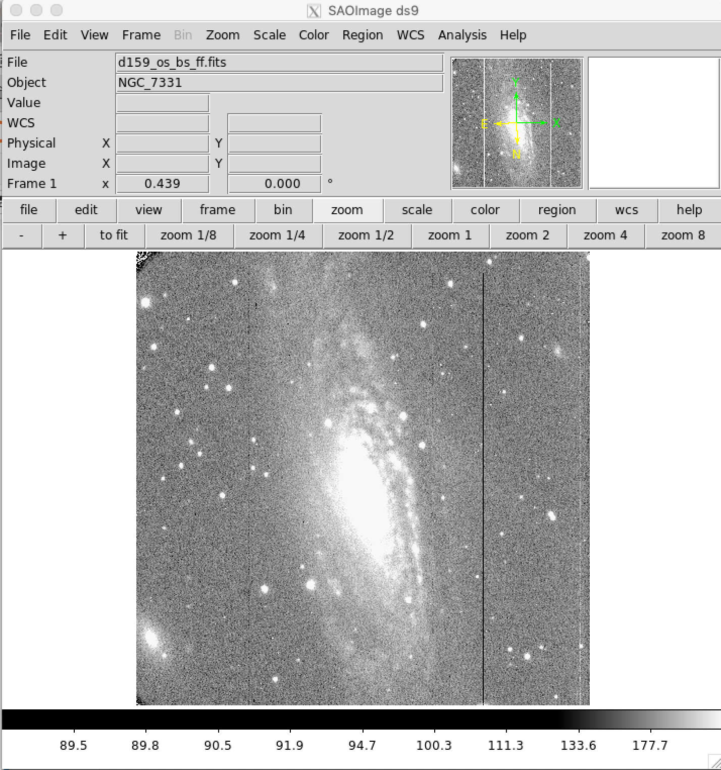
It is highly recommended to examine all the images after flat fielding to be sure that the flat field correction has been done propertly. The image below shows a properly flat fielded image.

Fix Known Bad Columns in Nickel CCD2 Images
The Nickel CCD2 detector has a number of known bad columns (easily seen in the flat fielded image above). These columns can be "fixed" by replacing them with the mean values of neighboring columns. First a bad pixel pixel mask is made highlighting the known bad columns. Then for each bad pixel, the mean of the surrounding good pixels is calculated and replaces the bad pixel. This procedure is somewhat time consuming, so be patient while it runs. Do not be alarmed if it gives a warning about converting mask elements to nan, as it still works correctly.
# Procedure to fix known bad columns in CCD2 images.  2016 Oct 2 E. Gates

# Create list of flat fielded data
datain =  glob2.glob(f2)

# _bp in output file name stands for bad pixel corrected
dataout = [i[:-5]+ '_bp.fits' for i in datain]

n=len(datain)
# size of box for area around bad pixel to be averaged
s=2

# read in one image to get image size for bad pixel mask
data,header=fits.getdata(datain[0],header=True)

# make bad pixel mask
mask=np.ma.make_mask(data,copy=True,shrink=True,dtype=np.bool)
mask[:,:]=False
mask[:,255:257]=True
mask[:,783:785]=True
mask[:,1001:1003]=True

# loop for all the data bad pixel correction
for k in range(0,n):
    data,header=fits.getdata(datain[k],header=True)
    mdata=np.ma.masked_array(data,mask=mask,fill_value=np.nan)
    dataFixed=data.copy()
    for i in range(0,mdata.shape[0]):
        for j in range(0,mdata.shape[1]):
            if np.math.isnan(mdata[i,j]):
                x1=i-s
                x2=i+s+1
                y1=j-s
                y2=j+s+1
                if x1<0:
                    x1=0
                if x2>mdata.shape[0]:
                    x2=mdata.shape[0]
                if y1<0:
                    y1=0
                if y2>mdata.shape[1]:
                    y2=mdata.shape[1]
                dataFixed[i,j]=np.mean(mdata[x1:x2,y1:y2])
    header['HISTORY']='Bad columns replaced'
    fits.writeto(dataout[k],dataFixed,header)
    # Move the now no longer needed files to archivedir
    basename=os.path.basename(datain[k])
    os.rename(datain[k],archivedir+basename)
Examine Bad Pixel Corrected Images
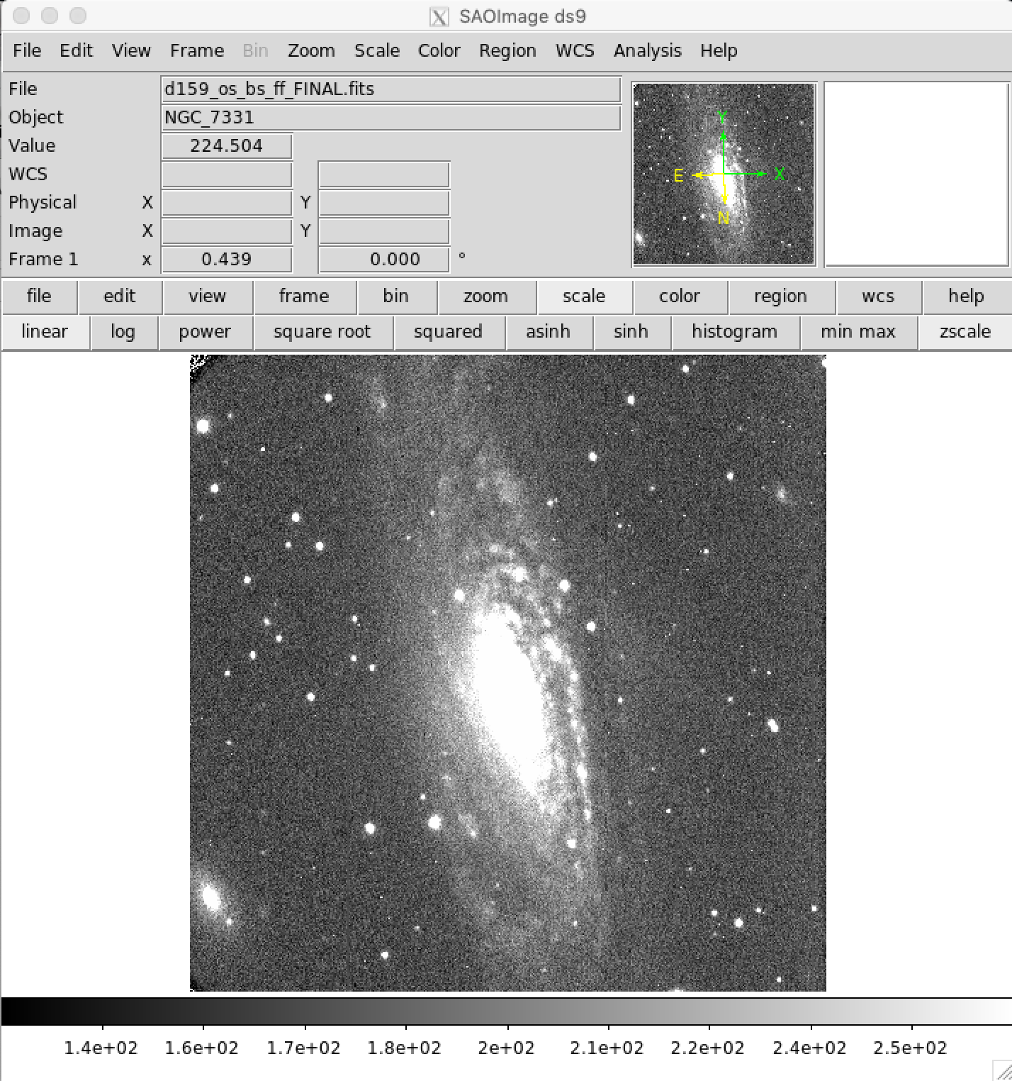
As always, it is good to check the pixel corrected images using DS9 or other image display tool. You can see in the image below that the bad columns were fixed reasonably well.

Cosmic Ray Removal
While the data probably look very good at this point, there are likely many cosmic rays contaminating the data. Removing all cosmic rays with software is difficult, but there are scripts that do a pretty good job. In this case we'll use the python module astroscrappy to do cosmic ray rejection. If you don't have astroscrappy installed, you'll want to install it using pip:
pip install astroscrappy
Note, it is not unusual to have to hand remove cosmic rays that are contaminating key pixels for data analysis, but that won't be covered in this jupyter notebook.
import astroscrappy

# Make a list of all the reduced data files
obs_list = glob2.glob(f2)
dataout = [i[:-5]+ '_crj.fits' for i in obs_list]
n=len(obs_list)
for i in range(0,n):
    data,header=fits.getdata(obs_list[i],header=True)
    data_fixed = data.copy()
    mask = np.ma.make_mask(data,copy=True,shrink=True, dtype=np.bool)
    mask[:,:] = False
    crmask,dataCR = astroscrappy.detect_cosmics(data_fixed,inmask=mask,cleantype='medmask')
    header['HISTORY'] = 'CR and bad pixels fixed with astroscrappy'
    fits.writeto(dataout[i],dataCR,header)
    # Move the now no longer needed files to archivedir
    basename=os.path.basename(obs_list[i])
    os.rename(obs_list[i],archivedir+basename)
Inspect Final Images
We have reached the end of the basic data reduction procedure where we have performed overscan subtraction, bias subtraction, flat field correction, removed the bad pixels in the CCD, and replaced cosmic ray hits. The saved final images can now be analyzed for whatever science goal is desired, e.g. astrometry or photometry.
Additional Python Resources and Tutorials
Python4Astronomers
http://python4astronomers.github.io/intro/intro.html
AstroPython Tutorials
http://www.astropython.org/tutorials/
astropy Tutorials
http://www.astropy.org/astropy-tutorials/
Python for Astronomers
http://www.iac.es/sieinvens/siepedia/pmwiki.php?n=HOWTOs.EmpezandoPython
Making Three Color Images with DS9
Now that you have the data reduced, you can make a pretty three color image. Basic usage of DS9 RGB frames is described in the following video.
https://www.youtube.com/watch?v=G77RcsAfMGM
Making Three Color Images with GIMP
Basic tutorial to make a three color images with GIMP.
Analyzing Data
Imexam is a convient tool based on IRAF IMEXAMINE. One can do aperture photometry, radial profile plots, FWHM measurements, etc. with this tool. Instructions for installation and use are available on-line at https://imexam.readthedocs.io/en/0.9.1/
Other photometry tools are part of the photutils python package (in fact some of the imexam procedures require photoutils). https://photutils.readthedocs.io/en/stable/